 Rohith's blog
The Quadratic form, Eigen Values, Curvature
Wed 14 December 2022Sree Rohith Pulipaka
The aim of this article is to relate the eigen values of hessian of the quadratic form with the curvature of the function to build an intuition between the two.
We consider the quadratic form
( 1 )
Where \(x \in R^{n},\ A\) is a Symmetric matrix. Specifically, if \(A\) is a positive definite matrix, each level set of equation ( 1 ) is the equations of an n-dimensional hyper ellipse (we shall see why).
Hessian of the quadratic form
( 2 )
Geometry of the quadratic form
We shall now look at why any level set of ( 1 ) is an n-dimensional hyper-ellipse. Firstly, the equation of an n-dimensional hyper-ellipse is
( 3 )
Where \(x_{i}\) is the \(i^{\text{th}}\) component of \(x\) and each \(a_{i}\) is the axis length of the ellipse in the \(\mathbf{e}_{\mathbf{i}}^{\text{th}}\) direction. Here \(\mathbf{e}_{\mathbf{i}}\) is the \(i^{\text{th}}\) canonical basis vector for \(R^{n}\). (For example, in \(R^{3}\), \(\mathbf{e}_{\mathbf{1}}\mathbf{= \ }\widehat{i},\ \mathbf{e}_{\mathbf{2}}\mathbf{=}\widehat{j},\mathbf{\ }\mathbf{e}_{\mathbf{3}}\mathbf{\ }\mathbf{=}\widehat{k}\)).
In 2 dimensions, \(a_{1},\ a_{2}\) are called the major and minor axes respectively. This hyper ellipse in ( 3 ) has it's axes parallel to the canonical directions. In other words, the ellipse is not tilted with respect to the coordinate plane.
Equation ( 3 ) can we re-written as follows:
( 4 )
Which looks a lot like our quadratic form ( 1 ). However, the matrix \(A\) in ( 1 ) need not be diagonal, but it needs to be positive definite for its level sets to represent an ellipse. Is there a way to get \(A\) into the diagonal form? Spectral Theorem to the rescue! For any symmetric matrix \(A\), we have an orthogonal matrix \(U\) and a diagonal matrix \(\Lambda\) such that
( 5 )
Substituting ( 5 ) in ( 1 ) and equating \(f\left( x \right) = 1\),
The \(\alpha\)-level set of \(f\left( x \right) = \left\{ \text{x } \right|f\left( x \right) = \ x^{T}Ax = \ \alpha\}\). Here for demonstration, we have selected \(\alpha = 1\).
If we let \(y = U^{T}x\), we see that we arrive at the same form as ( 4 ):
( 6 )
This is the standard form of the ellipse in the new variable \(y\). But what does \(y = U^{T}x\) represent? It represents a rotation of coordinates from old coordinates \(x\) to new coordinates \(y\).
Why? If we recall, rotation matrices are orthogonal, and their determinant is 1.
Definition of an orthogonal matrix: If \(U\) is an orthogonal matrix, \(UU^{T} = \ U^{T}U = I\) . This means that \(det(U)\) could be \(\pm 1 \Rightarrow\) Rotational Matrices are a subset of the set of Orthogonal matrices.
We now need to show that we can pick a \(U\) in ( 5 ) whose determinant is 1. (We can pick a \(U\) because spectral theorem does not say that it is unique, only that it is orthogonal.)
If we end up picking a \(U\) such that \(\det\left( U \right) = - 1\), form matrix
. Then, we can see that \(A = V\Lambda V^{T}\). Thus \(V\) is also allowed as the orthogonal matrix in ( 5 ). Therefore, we can pick a U which represents a rotation matrix and hence \(y = U^{T}x\) represents rotation of coordinates. This means that in the rotated(new) coordinates, our hyper ellipse is parallel to the new canonical directions This then means that in the untransformed coordinates (variable \(x\)), the axes of the hyper-ellipse are not parallel to the canonical directions \(\mathbf{e}_{\mathbf{i}}\).
Now we shall take the last step of this article: see the relation between the eigen values of \(A\) and curvature of \(f(x)\)!
Relation between curvature and hessian
We are almost there. Comparing ( 6 ) with ( 5 ), we also see that the lengths of the axes of the ellipse are equal to the inverse of the square root of the eigen value, i.e.
( 7 )
For \(\alpha \neq 1,\) the axes lengths scale by \(\alpha\). Therefore, it the eigen values of \(A\) are similar in value to each other, hyper-ellipse of each level-set will be less skewed and looks like a hyper-sphere, since axes lengths are similar and vice-versa.
Consider two cases such that \(A = A_{1}\) and \(A = A_{2}\) where the eigen values of \(A_{1}\) are large and that of \(A_{2}\) are small. This inturn means that for the same \(\alpha\)-level set, the axes lengths of the quadratic form with \(A_{1}\) are small and that of \(A\_ 2\) are large, due to ( 7 ). This implies that the quadratic form wit \(A_{1}\) is a steeper bowl than the quadratic form with \(A_{2}\).
Thus, if \(A\) has large eigen values, \(f(x)\) given by ( 1 ) is steeper that if it had smaller eigenvalues!
Examples:
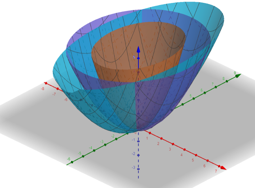
 Images generated on https://www.geogebra.org/calculator.
Each of the functions here is a quadratic form in
\(R^{2},\ x \in R,\ y \in R\). Use ( 3 ) to see it in the vector form. The
matrix A for each of these examples is indeed a diagonal matrix. For a
diagonal matrix, the eigen values are the values on the diagonal itself.
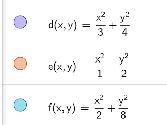
So for example, the values for \(d(x,y)\) are
\(\lambda_{1} = \frac{1}{3},\ \lambda_{2} = \frac{1}{4}\). We can see the
inverse relationship between the steepness of the function and its eigen
values.
Images generated on https://www.geogebra.org/calculator.
Each of the functions here is a quadratic form in
\(R^{2},\ x \in R,\ y \in R\). Use ( 3 ) to see it in the vector form. The
matrix A for each of these examples is indeed a diagonal matrix. For a
diagonal matrix, the eigen values are the values on the diagonal itself.
So for example, the values for \(d(x,y)\) are
\(\lambda_{1} = \frac{1}{3},\ \lambda_{2} = \frac{1}{4}\). We can see the
inverse relationship between the steepness of the function and its eigen
values.
For an interactive demonstration of eigen values, checkout: https://demonstrations.wolfram.com/EigenvaluesCurvatureAndQuadraticForms/. Hope this article helps you predict the function shape based on the matrix \(A\) even before you plot it!